Cubemaps

I know we talked about mimicking the real-life physics to achieve the fisheye lens effect. I suppose to that affect I could say there’s no rule that says the first pass has to be ready for human consumption. Nature doesn’t have to be either!

Last week we proved how it would be impossible to create a second pass that could sample a 2D first pass and achieve any semblance of quality. The view angle gets too steep:

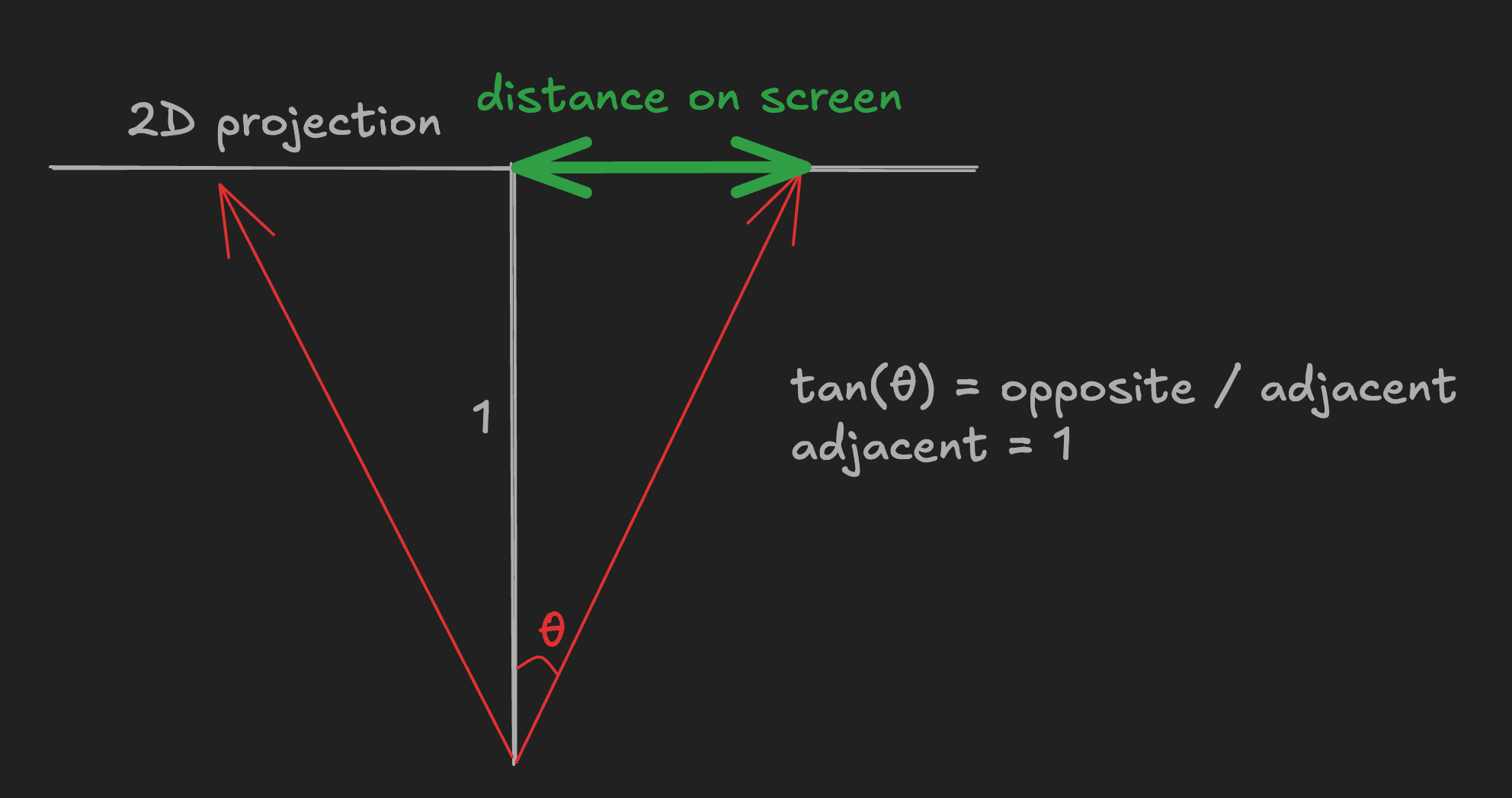
Therefore, the only place we can tackle this is in the first pass. How could we improve the viewing angle? Well, we could bend the projection!

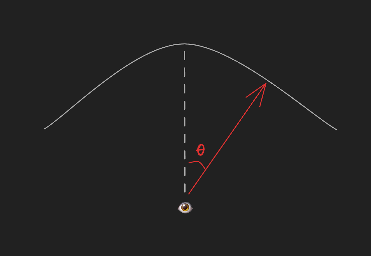
That sounds complicated though. (I realize I’m saying that after taking derivatives of trigonometric functions, but if nothing else we want to avoid the computer doing extra work!) What if…we just put in two sharp bends instead?

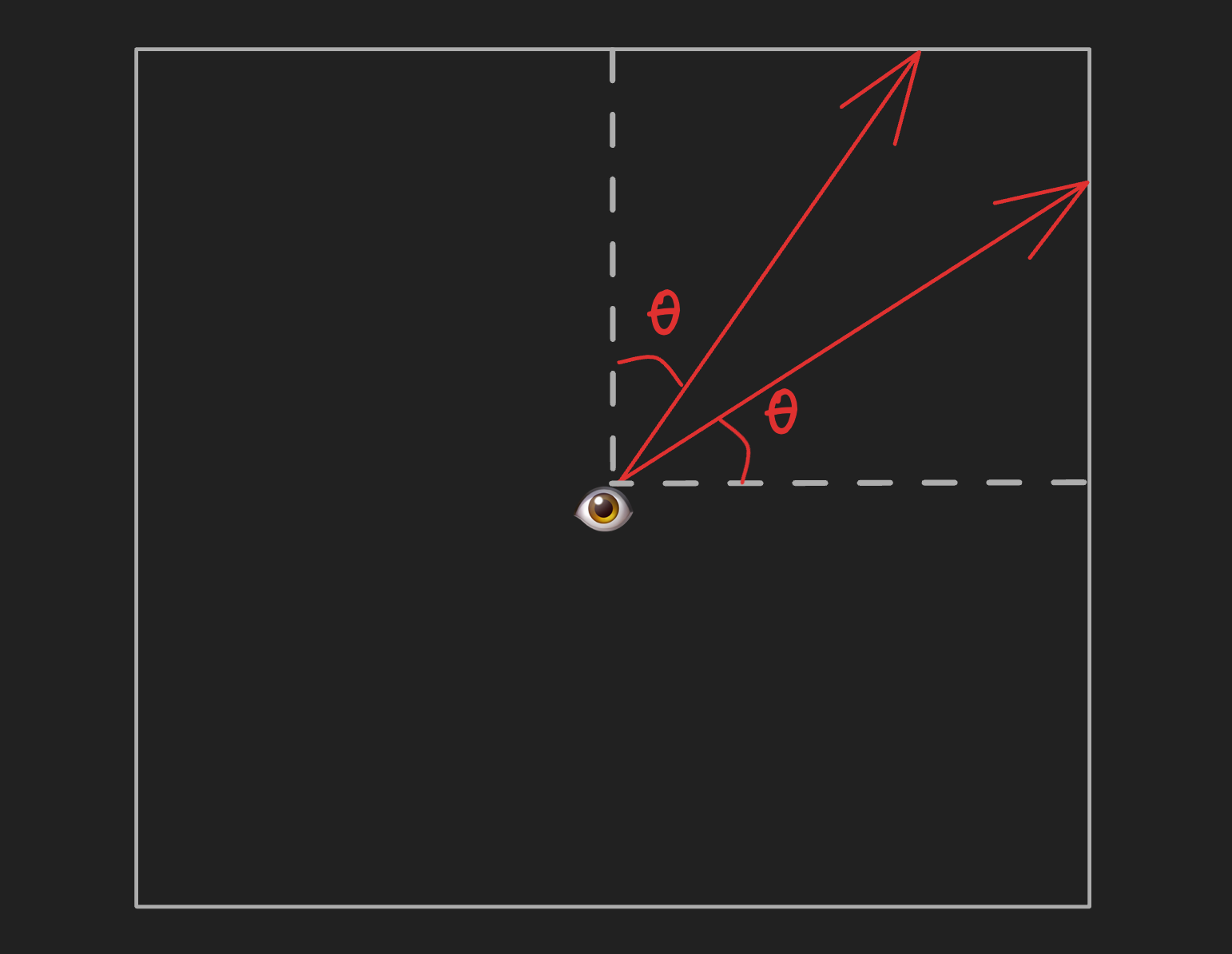
Add above and below to the equation and this, my friends, is the beginnings of a cubemap projection! Instead of mapping things continuously, anything in the first pass that would fall out of a (half) viewing angle θ of 45° is mapped onto the next square.

Our widest viewing angle, the trickiest place to sample, is now the corner of our cube. Our sample rate of change (that trigonometric derivative) sec²(θ), looking at the corner of our cube at 45° (a.k.a. π/4), does not approach infinity— sec²(π/4) is simply…2!

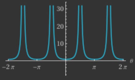
So at worst, we’ll need to sample at two times the sample rate at dead center. Perhaps a little challenging, but much more manageable than infinite.

And that’s what got a rendering like this:

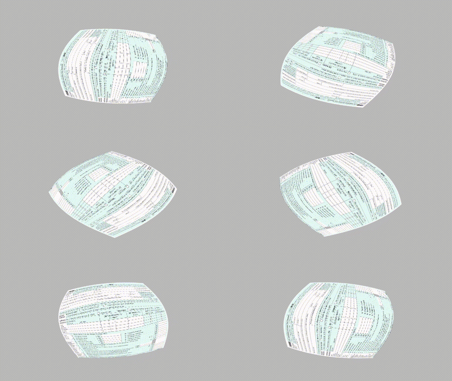
To look like this!

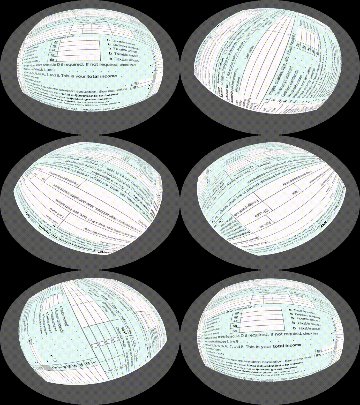
And with that out of the way, we’ll be able to move on to talking about the fisheye lens math itself!